qgis-pan-europeo

Pan European Proof of Concept

• Quick start
• How to use
  • Raster configuration
• Video tutorials
• About us

This QGIS plugin allows easy Multi Criteria Decision Analysis by creating a risk or priority summary raster, based in several arbitrary variables (rasters) with different units (e.g. population density, fuel load, etc.).

Users should define the variables to include, their relative weights, the utility attribute function, with its parameters; to standardize and weight-sum their values. In this way, users can compare totally different criteria (with different units or sense).

It also allows to define a study area by selecting a polygon (e.g. NUTS, LAU) or selecting the extent of the analysis in a easy and interactive way.

It runs entirely in the background, and by chunks; so users can continue working while the plugin calculates the results, without freezing their computer even with larger than RAM data. The backend is GDAL based and wrapped inside a QGIS processing plugin, so it is fast, efficient and integrable within a QGIS workflow.

Basic User Interface	Interface with Advanced Options Enabled

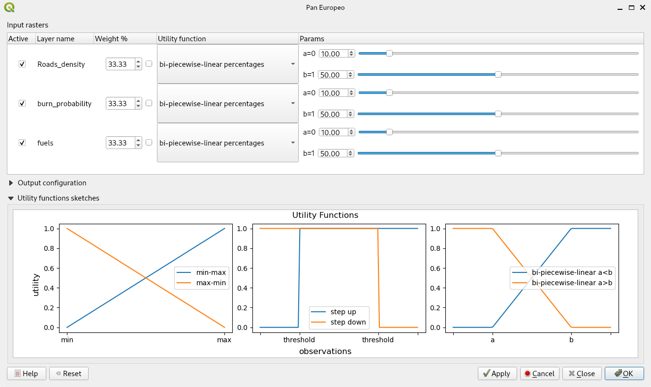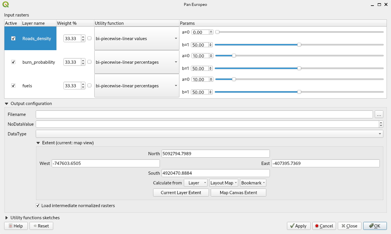Quick start

• Install QGIS (latest desktop version from qgis.org)
• In the QGIS menu, go to Plugins > Manage and Install Plugins
• All (vertical tab on the left) > Search for “Pan Europeo” in the top horizontal search bar > Select the plugin (checkbox) > Click “Install” (bottom right). A suggestion to install “Pan Europeo Processing” should be acknowledged, this is the dependency plugin that provides the backend for the “Pan Europeo” plugin.
• The plugin will be available in the “Plugins” section of the toolbar or in the “Plugins” menu, by clicking on the icon:

Plugin Icon

• Check out the below

How to use

1. Setup a QGIS Project
   a. Set the project CRS to EPSG:3857. Your raster layers should be in the same CRS.
   b. [Optional] Open the log panel (View > Panels > Log Messages) to read the plugin’s progress on the “PanEuropeo” tab.
2. Load a set of raster layers. Layers must be local and written to disk (GTiff is most reliable format).
3. [Optional] Load (a) Polygon(s) containing the study area.
4. Save the project.
5. Click on the “Pan European” plugin icon.
6. [Optional] Select a polygon feature to define the area of study. Click the “Apply” button to recalculate the parameter range values (min and max) of the new study area.
7. Configure for each layer/row weight and utility function (see details below)
8. [Optional] Configure target raster creation (only for advanced options mode).
   a. Filename: name and place where you will save the resulting layer (prioritization). If it is empty a temporary file will be generated.
   b. NoDataValue: Value to be used for pixels with no data.
   c. DataType: Data Type to be used for the resulting layer (prioritization).
9. Buttons:

   Help: Open this user manual.
   Reset: to clear the dialog, load another set of layers.
   Apply: redistributes the weights values so that they add up to 100
   Cancel: to close the dialog and do nothing.
   Ok: to calculate and get the results (priorization).
   

   After clicking “Ok” calculations will begin.
   Then a new, randomly named GTiff raster, will be written into your temporal files.
   It can be easily export as a pdf, png or other format by right click on the layer > Export > Save as [Image]

Raster configuration

For each available layer (must be local and saved/written to disk), available configurations are:

1. Layer enable/disable checkbox
2. Weight attributes as spinbox & slider (they get adjusted to sum 100 at run time)
3. Utility function configuration, select between:
   a. Min-Max scaling.
   b. Max-Min scaling, same as above, but inverted.
   c. Bi-Piecewise-Linear Values, with its two breakpoint setup as data real values.
   d. Bi-Piecewise-Linear Percentage, with its two breakpoint setup as percentage values from real data range (data.max - data.min).
   e. Step-Up value function, with a single breakpoint setup as data real value.
   f. Step-Up percentage function, with a single breakpoint setup as percentage.
   g. Step-Down value function, with a single breakpoint setup as data real value.
   h. Step-Down percentage function, with a single breakpoint setup as percentage.

Notice that for the Bi-Piecewise-Linear functions (c. and d.) crossing the breakpoints will invert the function’s slope.
Also in the case that one of them being zero (or minimun observation) a flat part is removed, e.g., a=0 and b>0:

You get up-slope and flat. Conversely, if b=0 and a>0, the graph will be reflected the vertically (as c. and d.), getting flat and down-slope.
Finally by one of them being 1 (or maximun observation) instead of 0, you get the other flat part removed.
If you choose to use the real values, please note that you may have to wait for QGIS to load the real values in the parameters section.

Known issues

• NoDataValues are converted to zero and used in the final weighted raster, allowing for much more datapoints than masking them out as the default GDAL calc behavior does, so be careful with your NoData values!
• Mixing different CRS will cause unexpected/untested results
• Currently different datatypes than Float-32 is untested

Video tutorials

Installation, easy from QGIS plugin manager, don’t forget Pan Europeo Processing dependency.

Project preparation, saved project, saved rasters, all written in local disk (not network or cloud) in the same projected CRS.

Navigation & await, selecting a study area triggers (cancellable) background tasks to update raster ranges.

Also triggered by manually input the extent group controller or by clicking “Map Canvas Extent” to set the current map view as study area.

About us

Role	Where	Method
Outreach	https://www.fire2a.com	fire2a@fire2a.com
User docs	https://fire2a.github.io/docs/	github-issues “forum”
Algorithms docs	https://fire2a.github.io/fire2a-lib/	Pull Requests
Developer docs	https://www.github.com/fire2a	Pull Requests

Developed by fdobad.82 @ Signal App Branding & testing by Felipe De La Barra felipedelabarra@fire2a.com

This site is open source. Improve this page.